White light CCF of HD 189733
In this notebook, we present a simple example of the application of the Doppler Shadow technique to ESPRESSO observations of HD 189733, a K1V star, extracting the white light CCF provided by the DRS.
[1]:
import numpy as np

from HECATE.HECATE import HECATE   # main class

from HECATE.get_data import *      # to retrieve the data
from HECATE.plots import *         # to plot the airmass and SNR
Warming up JIT-compiled functions...
Below we list the stellar, planetary and orbital parameters, as used in Cristo et al. (2024) and Gonçalves et al. (2026).
[2]:
stellar_params = {
                "Teff":4969, "Teff_err":43,   #effective temperature [K]
                "logg":4.60, "logg_err":0.01, #superficial gravity [dex]
                "FeH":-0.07, "FeH_err":0.02,  #metallicity [dex]
                "P_rot":2.21857312,           #rotation period [d]
                "R_star":0.766,               #radius [solar radii]
                "inc_star":71.87              #stellar inclination [º]
                }

planet_params = {
                "P_orb":2.21857312,           #orbital period [d]
                "a_R":8.76863,                #system scale [stellar radii]
                "Rp_Rs":0.1602,               #planet-to-star radius ratio
                "t0":53988.30339,             #mid-transit time [d]
                "e":0,                        #orbital eccentricity
                "w":90,                       #argument of periastron [º]
                "inc_planet":85.465,          #planet inclination [º]
                "lbda":-1.00,                 #spin-orbit angle [º]
                "dfp": -0.002424              #mid-transit phase shift, night of 2021-09-11
                }
Now we extract the CCFs from the example data provided.
[3]:
CCFs, time, airmass, berv, bervmax, snr, list_ccfs = get_CCFs(planet_params, stellar_params,
                                                              day='2021-08-11',
                                                              directory_path="HD189733_ESPRESSO_white_light_ccfs")
Need to download 11 files, approximately 3.67 MB
[4]:
plot_air_snr(planet_params, stellar_params, time, airmass, snr)
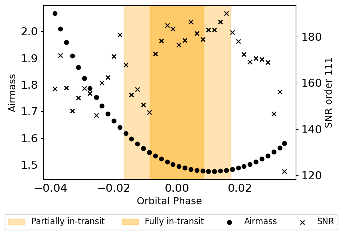
Now we call an instance of HECATE, giving the parameters and data, where the simulation of the transit with SOAP will take place.
[5]:
hecate = HECATE(planet_params, stellar_params, time, CCFs, spectra=None, plot_soap="SOAP")
To extract the local CCF, we just need to select the model to fit, the CCF type and the options for plotting.
[6]:
plot = {"fits_initial_CCF":False,         # plot the initial fits to the CCFs
        "sys_vel_ccf":True,               # plot the systemic velocity of the star in the CCFs
        "avg_out_of_transit_CCF":False,   # plot the average out-of-transit CCF
        "local_CCFs":True,                # plot the local CCFs
        "photometrical_rescale":False     # if the local CCFs are rescaled by the photometric transit model
        }

ccf_type = "white light"
model_fit = "modified Gaussian"
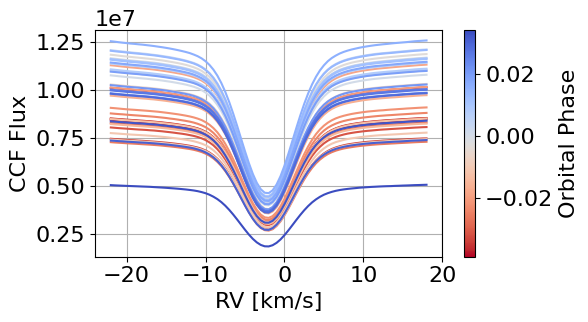
[7]:
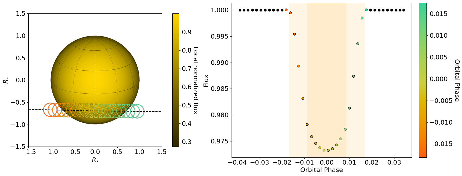
local_CCFs, CCFs_flux_corr, CCFs_sub_all, avg_out_of_transit_CCF = hecate.extract_local_CCF(model_fit, plot, save=None)
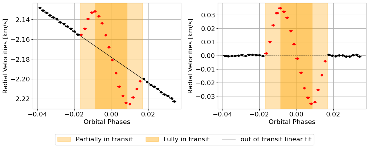
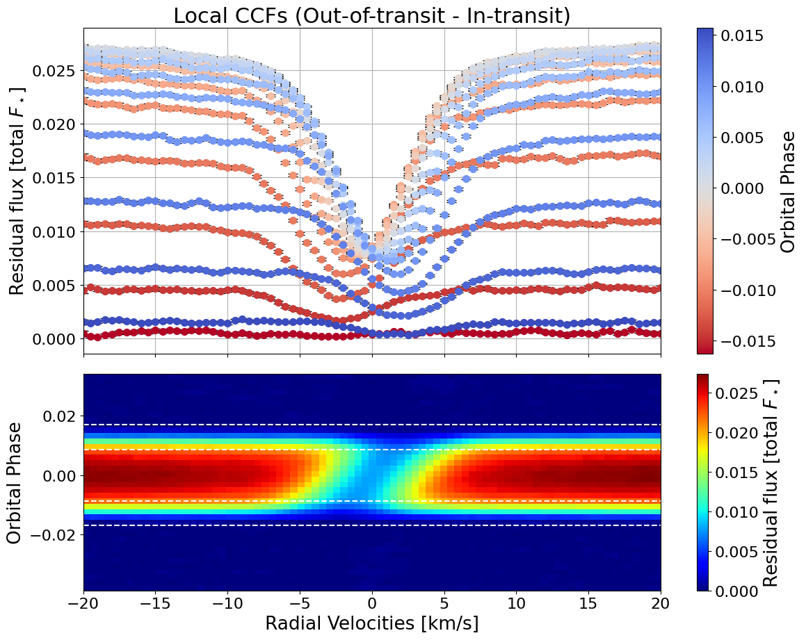
Tah-dah! We have the local white-light CCFs.
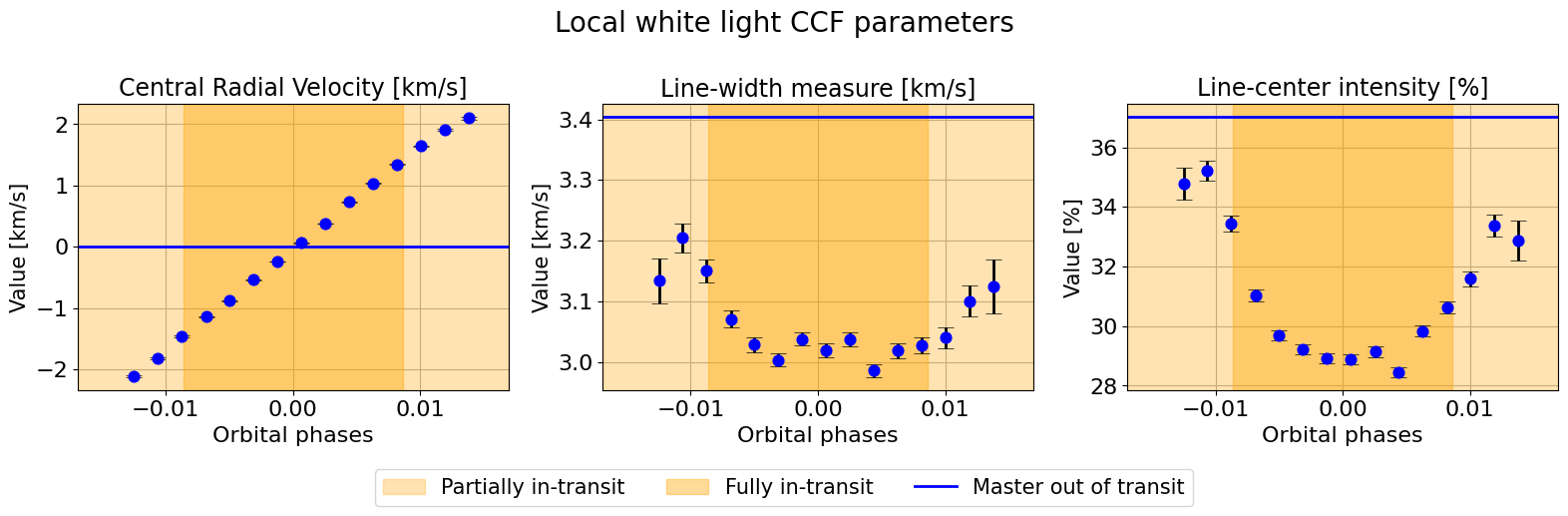
Now we can use HECATE to fit a profile to them, and extract the local parameters (central RV, line-center intensity, line-width measure) in function of \(\mu\) or \(\phi\).
[8]:
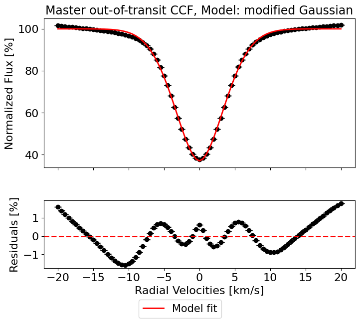
master_results = hecate.get_profile_parameters(profiles=avg_out_of_transit_CCF,
                                               data_type="CCF",
                                               observation_type="master",
                                               model="modified Gaussian",
                                               print_output=True,
                                               plot_fit=True)
##################################################
Fitting modified Gaussian model to master CCF profile
--------------------------------------------------
Fit parameters:
y0 = 0.999702 ± 0.000005
x0 = -0.000370 ± 0.000049
sigma = 3.404458 ± 0.000090
a = 0.629534 ± 0.000011
c = 1.823698 ± 0.000085
R^2:  0.9983
--------------------------------------------------
Profile parameters:
Central RV [km/s]: -0.000370 ± 0.000049
Continuum: 0.999702 ± 0.000005
Line-center intensity [%]: 37.027842 ± 0.001098
Line-width measure [km/s]: 3.404458 ± 0.000090
[9]:
local_results = hecate.get_profile_parameters(profiles=local_CCFs,
                                              data_type="CCF",
                                              observation_type="local",
                                              model="modified Gaussian",
                                              print_output=False,
                                              plot_fit=False)
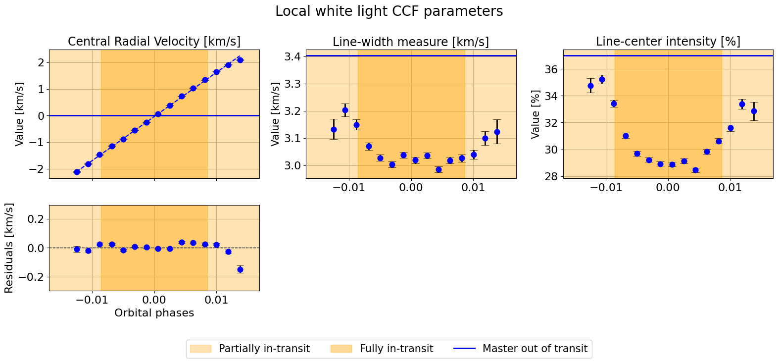
Having all the fits, we select the data based on quality – \(R^2 > 0.95\) and \(\mu \geq 0.3\).
[10]:
indices_final = np.array(list(set(np.where(local_results['R2'] >= 0.95)[0]).intersection(set(np.where(hecate.mu_in >= 0.3)[0]))))

local_params = [local_results['central_rv'], local_results['width'], local_results['intensity']]
master_params = [master_results['central_rv'], master_results['width'], master_results['intensity']]

hecate.plot_local_params(indices_final, local_params, master_params, suptitle=r"Local white light CCF parameters")
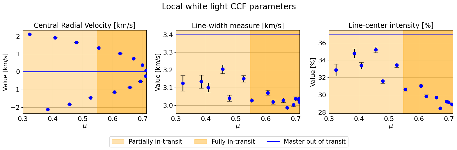
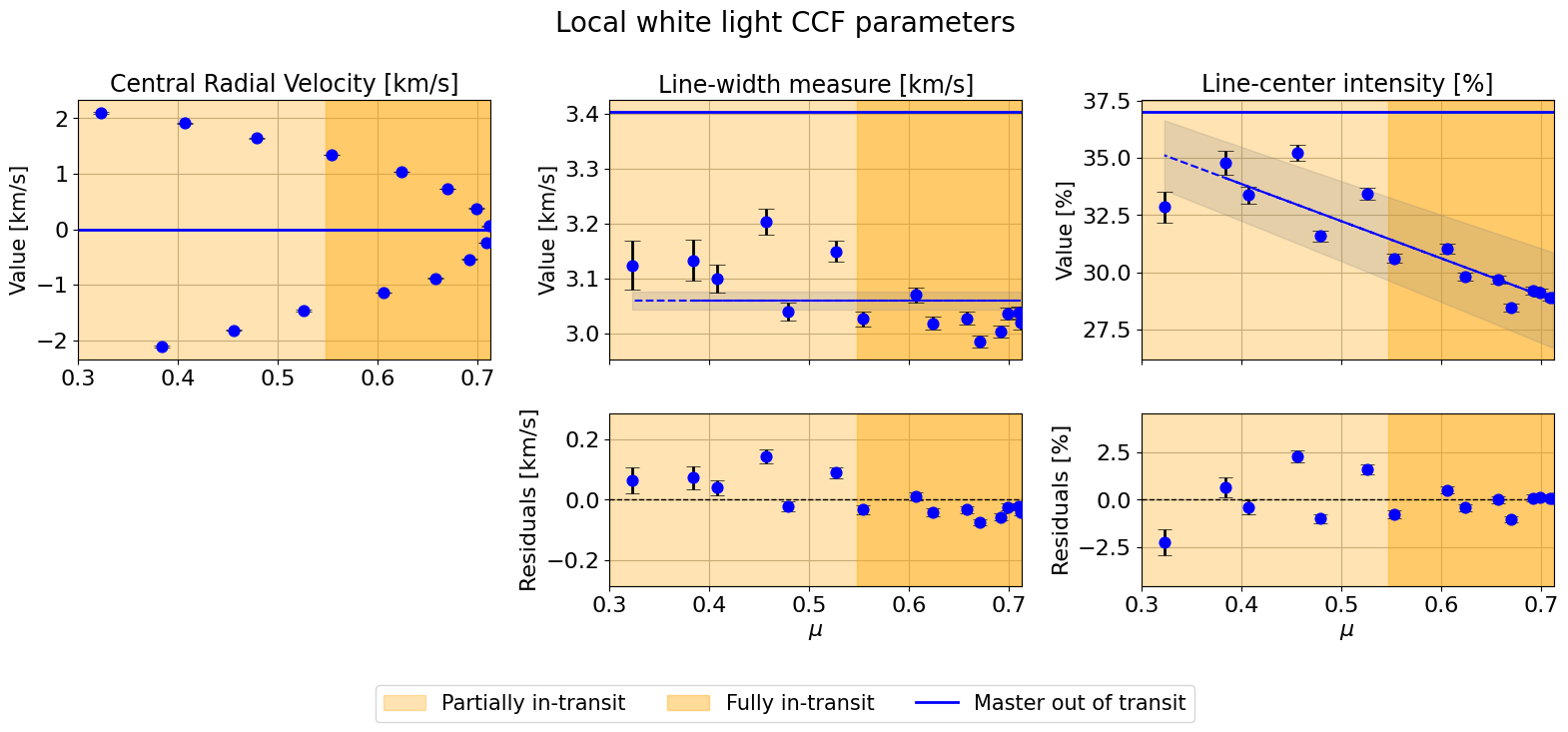
We can fit a linear model via nested sampling by running the same function.
[11]:
hecate.plot_local_params(indices_final, local_params, master_params,
                         suptitle=r"Local white light CCF parameters",
                         linear_fit_pairs=[("phases", 0), ("mu", 1), ("mu", 2)])
==================================================
Central Radial Velocity [km/s]
----------------------------------------
Orbital phases
18993it [00:29, 650.55it/s, batch: 7 | bound: 4 | nc: 1 | ncall: 391942 | eff(%):  4.714 | loglstar: 41.236 < 46.452 < 45.799 | logz: 29.987 +/-  0.110 | stop:  0.916]
14145it [00:18, 780.53it/s, batch: 7 | bound: 4 | nc: 1 | ncall: 268296 | eff(%):  5.074 | loglstar: -18.083 < -12.556 < -12.929 | logz: -19.675 +/-  0.071 | stop:  0.964]
------------------------------
Linear vs Constant
logZ(linear)   = 29.984 ± 0.102
logZ(constant) = -19.671 ± 0.063
log Bayes factor = 49.656
Unconstrained model favored.
------------------------------
18296it [00:27, 665.05it/s, batch: 6 | bound: 3 | nc: 1 | ncall: 375704 | eff(%):  4.731 | loglstar: 41.399 < 46.446 < 45.499 | logz: 30.228 +/-  0.110 | stop:  0.961]
16886it [00:23, 715.18it/s, batch: 6 | bound: 4 | nc: 1 | ncall: 341569 | eff(%):  4.789 | loglstar: -18.540 < -11.295 < -13.634 | logz: -22.513 +/-  0.086 | stop:  0.824]
Positive vs Negative slope
===========================
logZ(m>0)  = 30.226 ± 0.103
logZ(m<0)  = -22.487 ± 0.081
log Bayes factor = -52.712
Positive slope favored.
==========================
Linear fit parameters:
m = 165.448755 +/- 1.385715
b = -0.037545 +/- 0.004534
ln_f = -3.518267 +/- 0.237248
------------------------------
==================================================
Line-width measure [km/s]
----------------------------------------
$\mu$
20353it [00:31, 645.81it/s, batch: 7 | bound: 4 | nc: 1 | ncall: 421457 | eff(%):  4.706 | loglstar: 35.289 < 40.563 < 40.130 | logz: 22.077 +/-  0.117 | stop:  0.895]
17365it [00:24, 701.10it/s, batch: 8 | bound: 3 | nc: 1 | ncall: 338183 | eff(%):  4.980 | loglstar: 29.890 < 34.744 < 34.157 | logz: 23.551 +/-  0.081 | stop:  0.875]
------------------------------
Linear vs Constant
logZ(linear)   = 22.072 ± 0.106
logZ(constant) = 23.560 ± 0.077
log Bayes factor = -1.488
Zero-slope model favored
========================
Linear fit parameters:
b = 3.060577 +/- 0.016679
ln_f = -3.951362 +/- 0.224722
------------------------------
==================================================
Line-center intensity [%]
----------------------------------------
$\mu$
17217it [00:26, 654.37it/s, batch: 7 | bound: 4 | nc: 1 | ncall: 350381 | eff(%):  4.764 | loglstar: -12.413 < -6.831 < -7.428 | logz: -18.762 +/-  0.091 | stop:  0.880]
15587it [00:22, 692.97it/s, batch: 8 | bound: 3 | nc: 1 | ncall: 300202 | eff(%):  5.017 | loglstar: -24.312 < -19.263 < -19.787 | logz: -26.990 +/-  0.067 | stop:  0.885]
------------------------------
Linear vs Constant
logZ(linear)   = -18.767 ± 0.084
logZ(constant) = -26.982 ± 0.063
log Bayes factor = 8.215
Unconstrained model favored.
------------------------------
17119it [00:23, 740.56it/s, batch: 6 | bound: 5 | nc: 1 | ncall: 347527 | eff(%):  4.775 | loglstar: -25.547 < -19.290 < -19.907 | logz: -31.150 +/-  0.095 | stop:  0.852]
16010it [00:23, 673.03it/s, batch: 6 | bound: 3 | nc: 1 | ncall: 322038 | eff(%):  4.807 | loglstar: -12.163 < -6.831 < -7.774 | logz: -18.304 +/-  0.091 | stop:  0.953]
Positive vs Negative slope
===========================
logZ(m>0)  = -31.150 ± 0.084
logZ(m<0)  = -18.297 ± 0.084
log Bayes factor = 12.853
Negative slope favored.
==========================
Linear fit parameters:
m = -16.232177 +/- 2.244465
b = 40.358456 +/- 1.342313
ln_f = -3.454620 +/- 0.228164
------------------------------