White light CCF of HD 189733 - two nights
In this notebook, we present a simple example of the application of the Doppler Shadow technique to two nights of ESPRESSO observations of HD 189733, a K1V star, extracting the white light CCFs provided by the DRS. The nights of observations were 11-08-2021 and 31-08-2021.
We run two different instances of HECATE and then use the multi_night_analysis class to combine the data.
[1]:
import numpy as np

from HECATE.HECATE import HECATE   # main class
from HECATE.get_data import *
from HECATE.multi_night_analysis import multi_night_analysis # to perform the multi-night analysis
Warming up JIT-compiled functions...
[2]:
stellar_params = {
                "Teff":4969, "Teff_err":43,   #effective temperature [K]
                "logg":4.60, "logg_err":0.01, #superficial gravity [dex]
                "FeH":-0.07, "FeH_err":0.02,  #metallicity [dex]
                "P_rot":2.21857312,           #rotation period [d]
                "R_star":0.766,               #radius [solar radii]
                "inc_star":71.87              #stellar inclination [º]
                }

planet_params = {
                "P_orb":2.21857312,           #orbital period [d]
                "a_R":8.76863,                #system scale [stellar radii]
                "Rp_Rs":0.1602,               #planet-to-star radius ratio
                "t0":53988.30339,             #mid-transit time [d]
                "e":0,                        #orbital eccentricity
                "w":90,                       #argument of periastron [º]
                "inc_planet":85.465,          #planet inclination [º]
                "lbda":-1.00,                 #spin-orbit angle [º]
                "dfp": -0.002424              #mid-transit phase shift, night of 2021-09-11
                }
Now we quickly run HECATE for the first night of observations, saving the local CCF parameters.
[3]:
CCFs, time, airmass, berv, bervmax, snr, list_ccfs = get_CCFs(planet_params, stellar_params,
                                                              day='2021-08-11',
                                                              directory_path="HD189733_ESPRESSO_white_light_ccfs",
                                                              plot=False)
[4]:
hecate11 = HECATE(planet_params, stellar_params, time, CCFs, spectra=None, plot_soap=False)
[5]:
plot = {"fits_initial_CCF":False, # plot the initial fits to the CCFs
"sys_vel_ccf":False, # plot the systemic velocity of the star in the CCFs
"avg_out_of_transit_CCF":False, # plot the average out-of-transit CCF
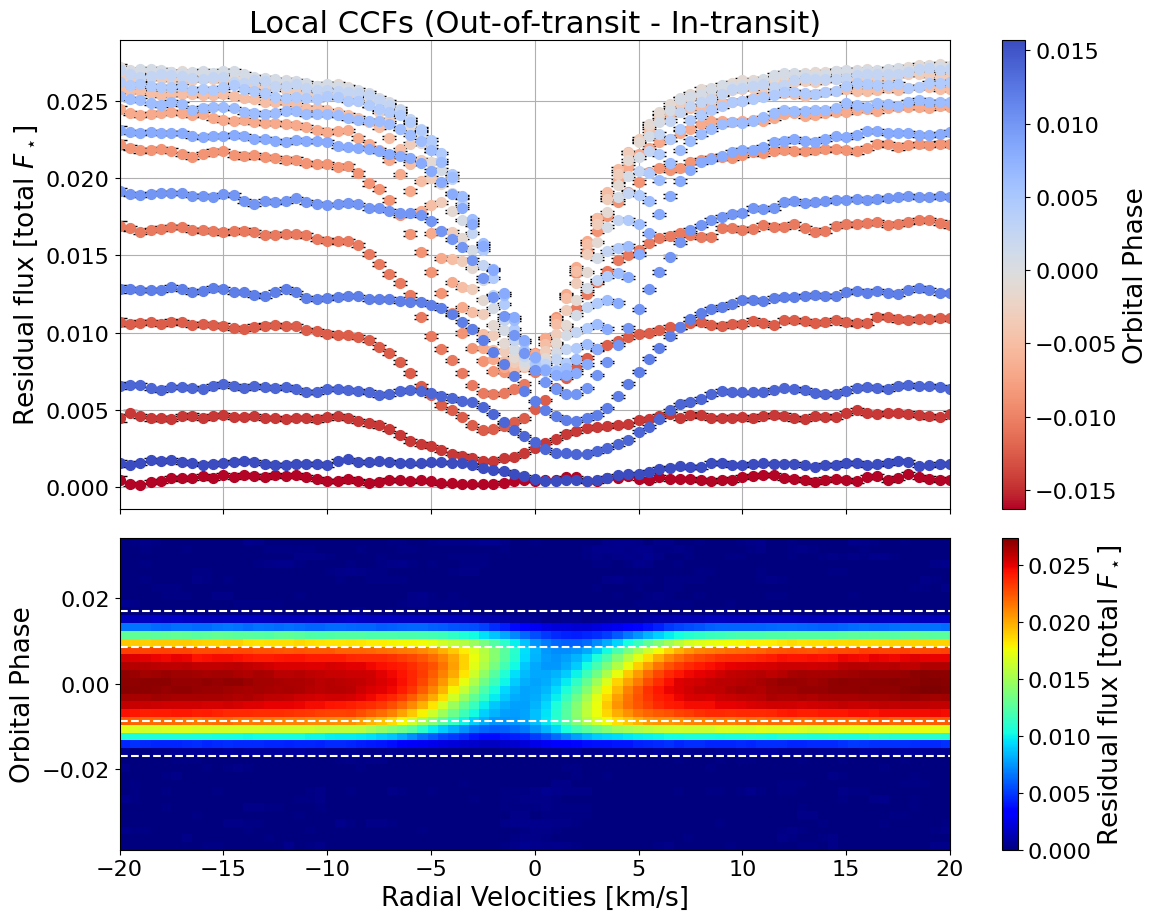
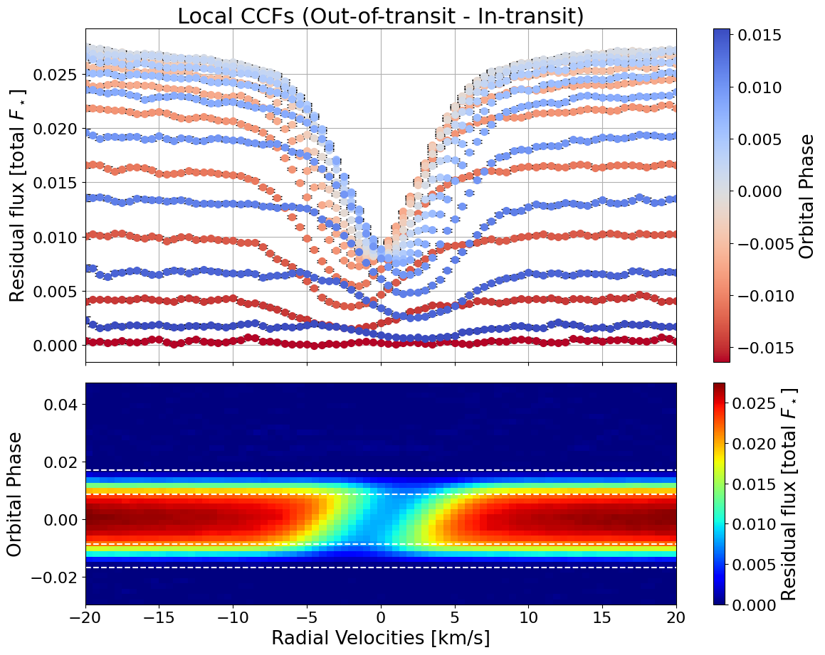
"local_CCFs":True, # plot the local CCFs
"photometrical_rescale":False # if the local CCFs are rescaled by the photometric transit model
}
ccf_type = "white light"
model_fit = "modified Gaussian"
[6]:
local_CCFs, CCFs_flux_corr, CCFs_sub_all, avg_out_of_transit_CCF = hecate11.extract_local_CCF(model_fit, plot, save=None)
[7]:
master_results11 = hecate11.get_profile_parameters(profiles=avg_out_of_transit_CCF,
                                               data_type="CCF",
                                               observation_type="master",
                                               model="modified Gaussian",
                                               print_output=False,
                                               plot_fit=False)
[8]:
local_results11 = hecate11.get_profile_parameters(profiles=local_CCFs,
                                              data_type="CCF",
                                              observation_type="local",
                                              model="modified Gaussian",
                                              print_output=False,
                                              plot_fit=False)
[9]:
indices_final11 = np.array(list(set(np.where(local_results11['R2'] >= 0.95)[0]).intersection(set(np.where(hecate11.mu_in >= 0.3)[0]))))

local_params11 = [local_results11['central_rv'], local_results11['width'], local_results11['intensity']]
master_params11 = [master_results11['central_rv'], master_results11['width'], master_results11['intensity']]
Now we do the same for the second night.
[10]:
planet_params["dfp"] = -0.002300 # mid-transit phase shift, night of 2021-08-31
[11]:
CCFs, time, airmass, berv, bervmax, snr, list_ccfs = get_CCFs(planet_params, stellar_params,
                                                              day='2021-08-31',
                                                              directory_path="HD189733_ESPRESSO_white_light_ccfs",
                                                              plot=False)
[12]:
hecate31 = HECATE(planet_params, stellar_params, time, CCFs, None)

plot = {"fits_initial_CCF":False,
        "sys_vel_ccf":False,
        "avg_out_of_transit_CCF":False,
        "local_CCFs":True,
        "photometrical_rescale":False}

ccf_type = "white light"
model_fit = "modified Gaussian"

local_CCFs, CCFs_flux_corr, CCFs_sub_all, avg_out_of_transit_CCF = hecate31.extract_local_CCF(model_fit, plot, save=None)
[13]:
master_results31 = hecate31.get_profile_parameters(profiles=avg_out_of_transit_CCF, data_type="CCF",
                                                    observation_type="master", model="modified Gaussian",
                                                    print_output=False, plot_fit=False)

local_results31 = hecate31.get_profile_parameters(profiles=local_CCFs, data_type="CCF",
                                                    observation_type="local", model="modified Gaussian",
                                                    print_output=False, plot_fit=False)
[14]:
indices_final31 = np.array(list(set(np.where(local_results31['R2'] >= 0.9)[0]).intersection(set(np.where(hecate31.mu_in >= 0.3)[0]))))

local_params31 = [local_results31['central_rv'], local_results31['width'], local_results31['intensity']]
master_params31 = [master_results31['central_rv'], master_results31['width'], master_results31['intensity']]
Having the results for each night, we build the following dictionaries:
[15]:
night_data_11 = {
    'hecate': hecate11,                             # HECATE instance
    'indices': indices_final11,                     # indices of points to retain
    'local_params': np.array(local_params11),       # local CCF parameters
    'master_params': np.array(master_params11),     # master CCF parameters
    'color': "blue",                                # color to use in the plots for this night
    'label': "2021-08-11"                           # label to use in the plots for this night
        }

night_data_31 = {
    'hecate': hecate31,
    'indices': indices_final31,
    'local_params': np.array(local_params31),
    'master_params': np.array(master_params31),
    'color': "red",
    'label': "2021-08-31"
        }
[16]:
night_data = {"2021-08-11": night_data_11,
              "2021-08-31": night_data_31}
[17]:
mult_night = multi_night_analysis(night_data, data_type='CCF')
We can just plot the two nights data in one single plot for each position parameter (\(\phi\) or \(\mu\)):
[18]:
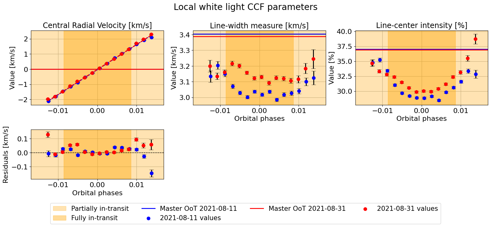
mult_night.plot_parameters(param_type='phases',
fit_each_night=False,
fit_combined=False,
combined_night_names=None,
plot_nested=False,
suptitle="Local white light CCF parameters")
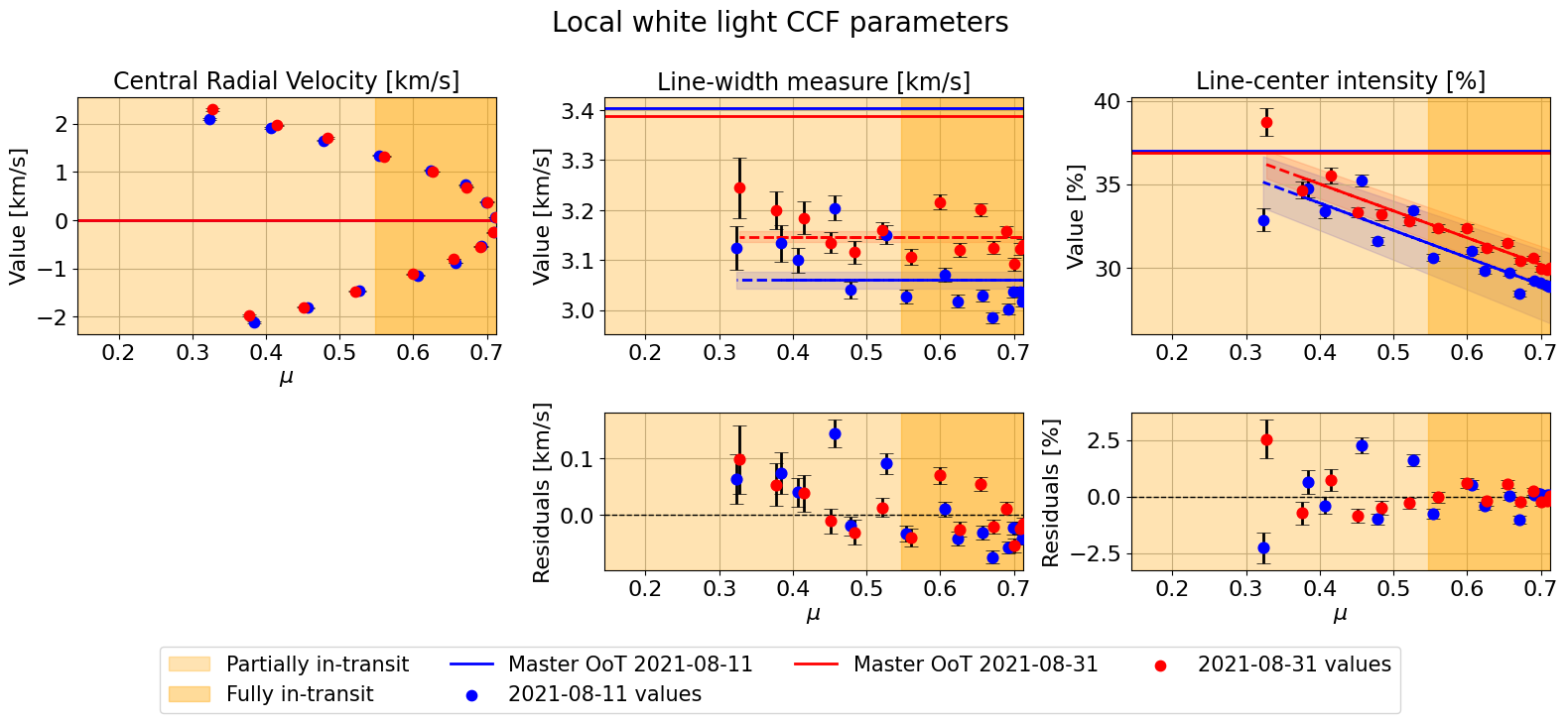
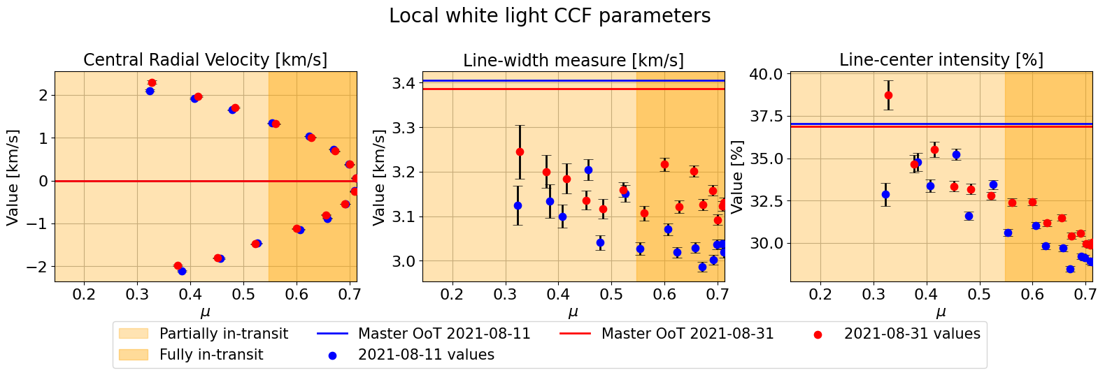
mult_night.plot_parameters(param_type='mu',
fit_each_night=False,
fit_combined=False,
combined_night_names=None,
plot_nested=False,
suptitle="Local white light CCF parameters")
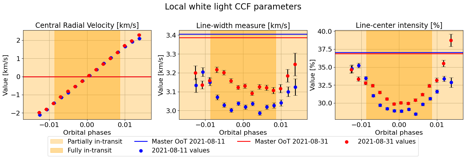
[18]:
{}
Or fit a linear model to each night:
[19]:
fit_results = mult_night.plot_parameters(param_type='phases',
                                      fit_each_night=True,
                                      fit_combined=False,
                                      fit_param_indices = np.array([0]),
                                      suptitle="Local white light CCF parameters")
21190it [00:31, 663.00it/s, batch: 7 | bound: 4 | nc: 1 | ncall: 442044 | eff(%):  4.677 | loglstar: 41.167 < 46.444 < 45.864 | logz: 26.002 +/-  0.124 | stop:  0.897]
17090it [00:22, 770.34it/s, batch: 7 | bound: 3 | nc: 1 | ncall: 332341 | eff(%):  4.985 | loglstar: -17.931 < -12.568 < -13.830 | logz: -24.281 +/-  0.087 | stop:  0.884]
------------------------------
Linear vs Constant
logZ(linear)   = 26.002 ± 0.113
logZ(constant) = -24.257 ± 0.083
log Bayes factor = 50.259
Unconstrained model favored.
------------------------------
21770it [00:33, 652.21it/s, batch: 7 | bound: 4 | nc: 1 | ncall: 455201 | eff(%):  4.670 | loglstar: 41.207 < 46.447 < 45.843 | logz: 24.882 +/-  0.127 | stop:  0.898]
17613it [00:24, 730.22it/s, batch: 5 | bound: 6 | nc: 1 | ncall: 359350 | eff(%):  4.756 | loglstar: -17.751 < -11.014 < -12.864 | logz: -27.839 +/-  0.125 | stop:  0.979]
Positive vs Negative slope
===========================
logZ(m>0)  = 24.878 ± 0.116
logZ(m<0)  = -27.826 ± 0.109
log Bayes factor = -52.704
Positive slope favored.
==========================
Linear fit parameters:
m = 165.446158 +/- 1.393267
b = -0.037505 +/- 0.004496
ln_f = -3.522776 +/- 0.232864
------------------------------
22094it [00:33, 655.36it/s, batch: 7 | bound: 4 | nc: 1 | ncall: 461484 | eff(%):  4.676 | loglstar: 38.304 < 43.603 < 43.184 | logz: 21.629 +/-  0.129 | stop:  0.890]
16351it [00:21, 758.91it/s, batch: 7 | bound: 4 | nc: 1 | ncall: 316766 | eff(%):  4.996 | loglstar: -17.750 < -12.542 < -13.195 | logz: -24.193 +/-  0.092 | stop:  0.940]
------------------------------
Linear vs Constant
logZ(linear)   = 21.645 ± 0.116
logZ(constant) = -24.186 ± 0.084
log Bayes factor = 45.832
Unconstrained model favored.
------------------------------
21821it [00:32, 664.49it/s, batch: 7 | bound: 4 | nc: 1 | ncall: 454749 | eff(%):  4.685 | loglstar: 38.395 < 43.597 < 43.144 | logz: 21.769 +/-  0.130 | stop:  0.901]
19592it [00:27, 719.54it/s, batch: 6 | bound: 7 | nc: 1 | ncall: 405877 | eff(%):  4.700 | loglstar: -18.435 < -10.892 < -12.594 | logz: -27.248 +/-  0.115 | stop:  0.783]
Positive vs Negative slope
===========================
logZ(m>0)  = 21.774 ± 0.117
logZ(m<0)  = -27.237 ± 0.103
log Bayes factor = -49.011
Positive slope favored.
==========================
Linear fit parameters:
m = 164.633395 +/- 1.720329
b = -0.020113 +/- 0.005087
ln_f = -3.285271 +/- 0.228280
------------------------------
[20]:
fit_results = mult_night.plot_parameters(param_type='mu',
                                      fit_each_night=True,
                                      fit_combined=False,
                                      fit_param_indices = np.array([1, 2]),
                                      suptitle="Local white light CCF parameters")
21858it [00:33, 659.64it/s, batch: 6 | bound: 3 | nc: 1 | ncall: 456539 | eff(%):  4.675 | loglstar: 35.622 < 40.547 < 39.524 | logz: 16.645 +/-  0.137 | stop:  0.980]
18196it [00:26, 694.17it/s, batch: 8 | bound: 3 | nc: 1 | ncall: 357714 | eff(%):  4.942 | loglstar: 30.035 < 34.704 < 34.135 | logz: 21.300 +/-  0.091 | stop:  0.891]
------------------------------
Linear vs Constant
logZ(linear)   = 16.623 ± 0.128
logZ(constant) = 21.296 ± 0.086
log Bayes factor = -4.673
Zero-slope model favored
========================
Linear fit parameters:
b = 3.060385 +/- 0.016268
ln_f = -3.952245 +/- 0.217799
------------------------------
21623it [00:33, 649.11it/s, batch: 6 | bound: 3 | nc: 1 | ncall: 451080 | eff(%):  4.679 | loglstar: 36.649 < 41.633 < 40.313 | logz: 18.027 +/-  0.136 | stop:  0.986]
18467it [00:26, 707.35it/s, batch: 8 | bound: 3 | nc: 1 | ncall: 362837 | eff(%):  4.946 | loglstar: 35.916 < 40.539 < 39.992 | logz: 26.156 +/-  0.095 | stop:  0.911]
------------------------------
Linear vs Constant
logZ(linear)   = 18.052 ± 0.128
logZ(constant) = 26.165 ± 0.090
log Bayes factor = -8.112
Zero-slope model favored
========================
Linear fit parameters:
b = 3.146783 +/- 0.010599
ln_f = -4.469513 +/- 0.243132
------------------------------
18897it [00:28, 667.12it/s, batch: 6 | bound: 3 | nc: 1 | ncall: 388140 | eff(%):  4.734 | loglstar: -11.811 < -6.828 < -7.786 | logz: -24.436 +/-  0.116 | stop:  0.961]
16923it [00:23, 715.63it/s, batch: 8 | bound: 3 | nc: 1 | ncall: 330222 | eff(%):  4.967 | loglstar: -24.259 < -19.277 < -19.580 | logz: -29.152 +/-  0.076 | stop:  0.875]
------------------------------
Linear vs Constant
logZ(linear)   = -24.450 ± 0.108
logZ(constant) = -29.140 ± 0.071
log Bayes factor = 4.690
Unconstrained model favored.
------------------------------
19234it [00:26, 730.64it/s, batch: 6 | bound: 3 | nc: 1 | ncall: 397422 | eff(%):  4.709 | loglstar: -25.259 < -19.422 < -20.906 | logz: -36.427 +/-  0.114 | stop:  0.876]
18231it [00:27, 673.87it/s, batch: 6 | bound: 4 | nc: 1 | ncall: 373274 | eff(%):  4.744 | loglstar: -11.935 < -6.820 < -7.220 | logz: -23.308 +/-  0.118 | stop:  0.981]
Positive vs Negative slope
===========================
logZ(m>0)  = -36.410 ± 0.107
logZ(m<0)  = -23.287 ± 0.105
log Bayes factor = 13.123
Negative slope favored.
==========================
Linear fit parameters:
m = -16.288863 +/- 2.245907
b = 40.390411 +/- 1.363256
ln_f = -3.459207 +/- 0.221864
------------------------------
20274it [00:30, 657.75it/s, batch: 7 | bound: 4 | nc: 1 | ncall: 420881 | eff(%):  4.694 | loglstar: -3.788 <  1.518 <  0.887 | logz: -17.367 +/-  0.119 | stop:  0.903]
16225it [00:22, 723.16it/s, batch: 8 | bound: 3 | nc: 1 | ncall: 314015 | eff(%):  5.000 | loglstar: -24.872 < -20.066 < -20.696 | logz: -29.942 +/-  0.078 | stop:  0.911]
------------------------------
Linear vs Constant
logZ(linear)   = -17.360 ± 0.110
logZ(constant) = -29.949 ± 0.074
log Bayes factor = 12.588
Unconstrained model favored.
------------------------------
20850it [00:28, 721.94it/s, batch: 7 | bound: 5 | nc: 1 | ncall: 434071 | eff(%):  4.685 | loglstar: -26.534 < -20.084 < -20.927 | logz: -37.472 +/-  0.112 | stop:  0.791]
19908it [00:30, 657.97it/s, batch: 7 | bound: 4 | nc: 1 | ncall: 412332 | eff(%):  4.703 | loglstar: -3.732 <  1.525 <  0.839 | logz: -16.525 +/-  0.116 | stop:  0.901]
Positive vs Negative slope
===========================
logZ(m>0)  = -37.467 ± 0.102
logZ(m<0)  = -16.539 ± 0.106
log Bayes factor = 20.929
Negative slope favored.
==========================
Linear fit parameters:
m = -16.079402 +/- 1.190150
b = 41.449304 +/- 0.737102
ln_f = -4.388216 +/- 0.347686
------------------------------